How Does Carbon Become Fossil Fuel Again
*For the new assessment of the terminal decade of agreement the carbon cycle, see the 2nd Country of the Carbon Wheel Report (2018).*
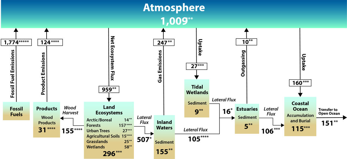
 emissions (red arrows); 2) uptake (black arrows); 3) lateral transfers (blue arrows); and 4) burial (blue arrows), which involves transfers of carbon from water to sediments and soils. Estimates—derived from Figure ES.3 and Figure 2.3 in Ch. 2: The North American Carbon Budget—are in teragrams of carbon (Tg C) per year. The increase in atmospheric carbon, denoted by a positive value, represents the net annual change resulting from the addition of carbon emissions minus net uptake of atmospheric carbon by ecosystems and coastal waters. The estimated increase in atmospheric carbon of +1,009 Tg C per year is from Figure 2.3 and that value is slightly different from the +1,008 Tg C per year value used elsewhere in Ch. 2 because of mathematical rounding. Net ecosystem carbon uptake represents the balance of carbon fluxes between the atmosphere and land (i.e., soils, grasslands, forests, permafrost, and boreal and Arctic ecosystems). Coastal waters include tidal wetlands, estuaries, and the coastal ocean (see Figure ES.3 for details). The net land sink, denoted by a positive value, is the net uptake by ecosystems and tidal wetlands (Figure ES.3) minus emissions from harvested wood and inland waters and estuar- ies (Figure ES.3). For consistency, the land sink estimate of 606 Tg C per year is adopted from Ch. 2. Because of rounding of the numbers in that chapter, this value differs slightly from the combined estimate from Figures ES.2 and ES.3 (605 Tg C per year). Asterisks indicate that there is 95% confidence that the actual value is within 10% (☆☆☆☆☆), 25% (☆☆☆☆), 50% (☆☆☆), 100% (☆☆), or >100% (☆) of the reported value. [Figure source: Adapted from Ciais et al., 2013, Figures 6.1 and 6.2; Copyright IPCC, used with permission.] Source: Second State of the Carbon Cycle Report 2018.")
What is the carbon cycle? What are the different pools and fluxes of carbon? Why are they of import? This page provides a compilation of data and relevant links to help respond some of these questions.
The Carbon Bicycle:What is the Carbon Bike? What is the fast and dull cycle and how are they influenced?
Carbon Measurement Approaches and Bookkeeping Frameworks: Approaches and methods for carbon stock and flow estimations, measurements, and bookkeeping
The N American Carbon Cycle: The latest (2018) cess and upkeep
Webinar Series Videos: 'The State of the Carbon Cycle: From Science to Solutions'
The Global Carbon Budget : The Global Carbon Upkeep equally calculated by a global group of scientists
Frequently asked questions and their answers:Answers to commonly asked questions such as the following are listed here: Can you quantify the sources and sinks of the global carbon cycle? How much carbon is stored in the different ecosystems? In terms of mass, how much carbon does i office per 1000000 by volume of atmospheric CO2 correspond? What pct of the CO2 in the atmosphere has been produced by human beings through the burning of fossil fuels?
 in gigatons (GT) (Source: U.S. Department of Energy Office of Science).")
The Carbon Cycle
(Original Source:NASA Earth Observatory)
'Carbon is the backbone of life on Globe. We are made of carbon, nosotros eat carbon, and our civilizations—our economies, our homes, our ways of transport—are built on carbon. We need carbon, simply that demand is as well entwined with one of the virtually serious problems facing us today: global climate change.....'
- What is the carbon cycle? 'Carbon flows between each reservoir in an exchange called the carbon cycle, which has irksome and fast components. Any alter in the wheel that shifts carbon out of i reservoir puts more carbon in the other reservoirs. Changes that put carbon gases into the atmosphere upshot in warmer temperatures on Earth....'
- The Slow Carbon Bicycle 'Through a series of chemical reactions and tectonic activity, carbon takes between 100-200 million years to move between rocks, soil, ocean, and atmosphere in the dull carbon cycle. On average, 1013 to 1014 grams (x–100 million metric tons) of carbon movement through the slow carbon cycle every yr. In comparison, human emissions of carbon to the atmosphere are on the lodge of 1015 grams, whereas the fast carbon cycle moves 1016 to 1017 grams of carbon per year....'
- The Fast Carbon Cycle: '...Plants and phytoplankton are the primary components of the fast carbon cycle. Phytoplankton (microscopic organisms in the ocean) and plants take carbon dioxide from the atmosphere past absorbing it into their cells. Using free energy from the Lord's day, both plants and plankton combine carbon dioxide (CO2) and h2o to form carbohydrate (CH2O) and oxygen. The chemic reaction looks similar this:
CO2 + H2O + energy = CH2O + O2
Iv things can happen to movement carbon from a constitute and return it to the atmosphere, merely all involve the aforementioned chemic reaction. Plants intermission downward the sugar to get the energy they need to grow. Animals (including people) eat the plants or plankton, and intermission down the plant saccharide to get free energy. Plants and plankton dice and decay (are eaten by leaner) at the terminate of the growing flavour. Or fire consumes plants. In each case, oxygen combines with sugar to release water, carbon dioxide, and free energy. The basic chemic reaction looks like this:
CH2O + Oii = COtwo + HiiO + energy
 depicts different biogeochemical cycles, including the carbon cycle, as influenced by different factors. 'The top panel shows the impact of the alteration of the carbon cycle alone on radiative forcing. The bottom panel shows the impacts of the alteration of carbon, nitrogen, and sulfur cycles on radiative forcing. SO2 and NH3 increase aerosols and decrease radiative forcing. NH3 is likely to increase plant biomass, and consequently decrease forcing. NOx is likely to increase the formation of tropospheric ozone (O3) and increase radiative forcing. Ozone has a negative effect on plant growth/biomass, which might increase radiative forcing. CO2 and NH3 act synergistically to increase plant growth, and therefore decrease radiative forcing. SO2 is likely to reduce plant growth, perhaps through the leaching of soil nutrients, and consequently increase radiative forcing. NOx is likely to reduce plant growth directly and through the leaching of soil nutrients, therefore increasing radiative forcing. However, it could act as a fertilizer that would have the opposite effect.' (National Climate Assessment, 2014)")
In all 4 processes, the carbon dioxide released in the reaction usually ends up in the temper. The fast carbon wheel is so tightly tied to constitute life that the growing season can exist seen by the way carbon dioxide fluctuates in the atmosphere. In the Northern Hemisphere winter, when few land plants are growing and many are decaying, atmospheric carbon dioxide concentrations climb. During the spring, when plants begin growing again, concentrations drop. It is as if the Earth is animate. The ebb and menstruum of the fast carbon bicycle is visible in the changing seasons. As the big country masses of Northern Hemisphere green in the jump and summer, they draw carbon out of the atmosphere. This graph shows the divergence in carbon dioxide levels from the previous month, with the long-term tendency removed. This cycle peaks in Baronial, with about 2 parts per one thousand thousand of carbon dioxide fatigued out of the temper. In the fall and winter, as vegetation dies back in the northern hemisphere, decomposition and respiration returns carbon dioxide to the atmosphere. These maps prove net primary productivity (the amount of carbon consumed by plants) on land (green) and in the oceans (blue) during August and December, 2010. In August, the green areas of North America, Europe, and Asia represent plants using carbon from the atmosphere to grow. In December, net primary productivity at high latitudes is negative, which outweighs the seasonal increment in vegetation in the southern hemisphere. Equally a result, the amount of carbon dioxide in the atmosphere increases....'
- Changes in the Carbon Cycle 'Left unperturbed, the fast and ho-hum carbon cycles maintain a relatively steady concentration of carbon in the atmosphere, land, plants, and ocean. But when annihilation changes the amount of carbon in one reservoir, the upshot ripples through the others....'
- Furnishings of Changing the Carbon Cycle 'It is significant that so much carbon dioxide stays in the atmosphere because COii is the most important gas for decision-making Earth'due south temperature. Carbon dioxide, methyl hydride, and halocarbons are greenhouse gases that absorb a wide range of energy—including infrared energy (rut) emitted past the Globe—and then re-emit it. The re-emitted energy travels out in all directions, but some returns to World, where it heats the surface. Without greenhouse gases, Earth would be a frozen -xviii degrees Celsius (0 degrees Fahrenheit). With likewise many greenhouse gases, Earth would exist similar Venus, where the greenhouse atmosphere keeps temperatures effectually 400 degrees Celsius (750 Fahrenheit)....'
- Studying the Carbon Cycle 'What will those changes look like? What will happen to plants as temperatures increase and climate changes? Will they remove more carbon from the atmosphere than they put back? Will they become less productive? How much extra carbon will melting permafrost put into the atmosphere, and how much will that dilate warming? Will ocean apportionment or warming change the rate at which the ocean takes upwardly carbon? Will body of water life become less productive? How much will the ocean acidify, and what effects will that have?....' (Original Source: NASA Earth Observatory)
Carbon measurement Approaches and Accounting Frameworks
From the Country of the Carbon Cycle Report (USGCRP, 2018) Preface (Shrestha et al, 2018):
'Three observational, analytical, and modeling methods are used to estimate carbon stocks and fluxes: 1) inventory measurements or "lesser-upward" methods, two) atmospheric measurements or "top-downwards" methods, and three) ecosystem models (run into Appendix D for details). "Bottom-upwardly" estimates of carbon exchange with the atmosphere depend on measurements of carbon contained in biomass, soils, and water, as well as measurements of COtwo and CHiv exchange among the land, h2o, and atmosphere. Examples include straight measurement of power plant carbon emissions; remote-sensing and field measurements repeated over fourth dimension to guess changes in ecosystem stocks; measurements of the amount of carbon gases emitted from land and water ecosystems to the atmosphere (in chambers or, at larger scales, using sensors on towers); and combined urban demographic and activeness information (e.g., population and building floor areas) with "emissions factors" to estimate the amount of CO2 released per unit of action.
Superlative-downward approaches infer fluxes from the terrestrial land surface and sea past coupling atmospheric gas measurements (using air sampling instruments on the ground, towers, buildings, balloons, and shipping or remote sensors on satellites) with carbon isotope methods, tracer techniques, and simulations of how these gases move in the temper. The network of GHG measurements, types of measurement techniques, and diversity of gases measured has grown exponentially since SOCCR1 (CCSP 2007), providing improved estimates of COii and CH4 emissions and increased temporal resolution at regional to local scales across N America.
Ecosystem models are used to judge carbon stocks and fluxes with mathematical representations of essential processes, such every bit photosynthesis and respiration, and how these processes answer to external factors, such as temperature, precipitation, solar radiation, and h2o move. Models too are used with top-down atmospheric measurements to attribute observed GHG fluxes to specific terrestrial or ocean features or locations.'
For details, see the SOCCR2 Preface (Shrestha et al. 2018) and Appendix D (Birdsey et al. 2018).
References:
Shrestha, 1000., North. Cavallaro, R. Birdsey, M. A. Mayes, R. G. Najjar, S. C. Reed, P. Romero-Lankao, Due north. P. Gurwick, P. J. Marcotullio, and J. Field, 2018: Preface. In 2d State of the Carbon Bicycle Report (SOCCR2): A Sustained Assessment Report [Cavallaro, N., Thousand. Shrestha, R. Birdsey, M. A. Mayes, R. K. Najjar, S. C. Reed, P. Romero-Lankao, and Z. Zhu (eds.)]. U.S. Global Change Enquiry Program, Washington, DC, Us, pp. 5-20, https://doi.org/10.7930/SOCCR2.2018.Preface.
Birdsey, R., N. P. Gurwick, K. R. Gurney, G. Shrestha, One thousand. A. Mayes, R. Yard. Najjar, S. C. Reed, and P. RomeroLankao, 2018: Appendix D. Carbon measurement approaches and accounting frameworks. In Second State of the Carbon Cycle Study (SOCCR2): A Sustained Cess Written report [Cavallaro, N., G. Shrestha, R. Birdsey, Thousand. A. Mayes, R. M. Najjar, S. C. Reed, P. Romero-Lankao, and Z. Zhu (eds.)]. U.South. Global Change Research Program, Washington, DC, USA, pp. 834-838, doi: https:// doi.org/x.7930/SOCCR2.2018.AppD.
Back to top
The N American Carbon Cycle and Budget
Excerpt from the Second State of the Carbon Cycle Report (SOCCR2, USGCRP 2018) Affiliate 2 (Hayes et. al, 2018):
'Since the Industrial Revolution, human activity has released into the atmosphere unprecedented amounts of carbon-containing greenhouse gases (GHGs), such as carbon dioxide (COtwo) and methyl hydride (CH4), that take influenced the global carbon cycle. For the by three centuries, North America has been recognized as a internet source of CO2 emissions to the temper (Houghton 1999, 2003; Houghton and Hackler 2000; Hurtt et al., 2002). At present there is greater interest in including in this film emissions of CH4 because it has 28 times the global warming potential of CO2 over a 100-year time horizon (Myhre et al., 2013; NAS 2018).
The major continental sources of COtwo and CH4 are 1) fossil fuel emissions, two) wildfire and other disturbances, and 3) land-use alter. Globally, continental carbon sources are partially kickoff by sinks from natural and managed ecosystems via plant photosynthesis that converts CO2 into biomass. The terrestrial carbon sink in North America is known to offset a substantial proportion of the continent's cumulative carbon sources. Although uncertain, quantitative estimates of this beginning over the final two decades range from as low as 16% to equally high as 52% (Rex et al., 2015). Highlighted in this chapter are persistent challenges in unravelling CH4 dynamics across North America that arise from the need to fully quantify multiple sources and sinks, both natural (Warner et al., 2017) and anthropogenic (Hendrick et al., 2016; Turner et al., 2016a; NAS 2018). Adding to the claiming is disagreement on whether the reported magnitudes of CH4 sources and sinks in the United States are underestimated (Bruhwiler et al., 2017; Miller et al., 2013; Turner et al., 2016a).
At the global scale, well-nigh 50% of almanac anthropogenic carbon emissions are sequestered in marine and terrestrial ecosystems (Le Quéré et al., 2016). Temporal patterns point that fossil carbon emissions accept increased from three.3 petagrams of carbon (Pg C) per year to almost 10 Pg C over the past fifty years (Le Quéré et al., 2015). Nevertheless, considerable uncertainty remains in the spatial patterns of emissions at finer scales over which carbon management decisions are fabricated. About importantly, the sensitivity of terrestrial sources and sinks to variability and trends in the biophysical factors driving the carbon bike is non understood well enough to provide good confidence in projections of the hereafter performance of the Due north American carbon residue (Friedlingstein et al., 2006; McGuire et al., 2016; Tian et al., 2016).'
For farther details, see the latest decadal assessment of N American Carbon Cyle, the Second Land of the Carbon Cycle Report.
References:
Hayes, D. J., R. Vargas, S. R. Alin, R. T. Conant, L. R. Hutyra, A. R. Jacobson, W. A. Kurz, Due south. Liu, A. D. McGuire, B. Poulter, and C. West. Woodall, 2018: Affiliate two: The North American carbon budget. In Second State of the Carbon Cycle Study (SOCCR2): A Sustained Assessment Report [Cavallaro, Northward., Chiliad. Shrestha, R. Birdsey, M. A. Mayes, R. Thousand. Najjar, S. C. Reed, P. Romero-Lankao, and Z. Zhu (eds.)]. U.S. Global Modify Research Plan, Washington, DC, USA, pp. 71-108, https://doi.org/ten.7930/SOCCR2.2018.Ch2.
USGCRP, 2018: 2nd State of the Carbon Cycle Study (SOCCR2): A Sustained Assessment Report. [Cavallaro, N., One thousand. Shrestha, R. Birdsey, Chiliad. A. Mayes, R. Thou. Najjar, S. C. Reed, P. Romero-Lankao, and Z. Zhu (eds.)]. U.S. Global Change Research Program, Washington, DC, United states of america, 878 pp., https://doi.org/x.7930/SOCCR2.2018
Back to top
Webinar Series Videos: 'The State of the Carbon Cycle: From Science to Solutions' and others
Recorded webinars describing what is the carbon wheel, focusing on the 2d Land of the Carbon Cycle Report scientific discipline findings and pertinent scientific and societally-relevant activities, are posted on our YouTube Channel. The series desciption is hither.

Dorsum to top
Global carbon budget
Note: For the latest annual global carbon and methyl hydride budgets, please see the Global Carbon Project.
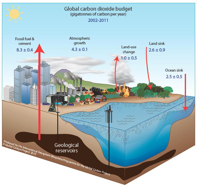
The adjacent effigy on the left represents recent global carbon budget estimates of annual carbon flows averaged from 2002 to 2011 , every bit provided in the Global Carbon Project's 2013 report. (Values in gigatons of carbon per year)
Notation:
1 GtC = 1 gigaton of carbon (or British-French onegigatonne of carbon)
= x 9 metric ton carbon or i billion tons of carbon
= i PgC = 1 petagram of carbon = 10 15 one thousand of carbon
ane metric ton = thou Kg = 10 6 g
(The metric ton is besides written as tonne in the British and French systems, every bit in this Global Carbon Upkeep figure.)
Back to top
Oftentimes asked questions and their answers about the carbon cycle
(Source: Carbon Dioxide Data Assay Center, CDIAC)
Q. What are the present tropospheric concentrations, global warming potentials (100 twelvemonth fourth dimension horizon), and atmospheric lifetimes of CO 2 , CH 4 , N two O, Chlorofluorocarbon-11, CFC-12, Chlorofluorocarbon-113, CCl 4 , methyl chloroform, HCFC-22, sulphur hexafluoride, trifluoromethyl sulphur pentafluoride, perfluoroethane, and surface ozone?
A. View a table presenting data and source for electric current greenhouse gas concentrations.
Q. Can you quantify the sources and sinks of the global carbon cycle?
A. Read a discussion of the global carbon cycle. You may also view the figures here (adapted by CDIAC from the IPCC 4th Assessment Written report: Climate change 2007 and the Woods Hole Research Center.)
Note: GtC = gigaton of carbon and giga = x9 and Pg C = petagram of carbon and Peta = 1015
Find the latest carbon budget estimates. Source: Global Carbon Projection
And, click hither to see figures summarizing the global cycles of biologically active elements. Source: William S. Reeburgh, Professor Marine and Terrestrial Biogeochemistry, University of California.
Q. How much carbon is stored in the different ecosystems?
A. View an illustration of the major earth ecosystem complexes ranked past carbon in live vegetation.
Q. In terms of mass, how much carbon does one part per one thousand thousand by volume of atmospheric CO 2 represent?
A. Using 5.137 x ten 18 kg as the mass of the atmosphere (Trenberth, 1981 JGR 86:5238-46), 1 ppmv of CO two = 2.13 Gt of carbon.
Back to pinnacle
Q. What percentage of the CO 2 in the atmosphere has been produced by human beings through the burning of fossil fuels?
A. Anthropogenic CO 2 comes from fossil fuel combustion, changes in land use (east.g., woods immigration), and cement manufacture. Houghton and Hackler accept estimated state-use changes from 1850-2000, then information technology is convenient to use 1850 as our starting signal for the post-obit give-and-take. Atmospheric CO 2 concentrations had not changed appreciably over the preceding 850 years (IPCC; The Scientific Basis) so information technology may exist safely assumed that they would not have inverse appreciably in the 150 years from 1850 to 2000 in the absence of human intervention.
In the following calculations, we will limited atmospheric concentrations of CO 2 in units of parts per million by volume (ppmv). Each ppmv represents two.13 X10 15 grams, or 2.xiii petagrams of carbon (PgC) in the atmosphere. Co-ordinate to Houghton and Hackler, land-use changes from 1850-2000 resulted in a net transfer of 154 PgC to the atmosphere. During that aforementioned menstruation, 282 PgC were released past combustion of fossil fuels, and v.5 additional PgC were released to the atmosphere from cement manufacture. This adds upwards to 154 + 282 + 5.v = 441.v PgC, of which 282/444.1 = 64% is due to fossil-fuel combustion.
Atmospheric CO ii concentrations rose from 288 ppmv in 1850 to 369.5 ppmv in 2000, for an increment of 81.v ppmv, or 174 PgC. In other words, about 40% (174/441.5) of the boosted carbon has remained in the atmosphere, while the remaining lx% has been transferred to the oceans and terrestrial biosphere.
The 369.5 ppmv of carbon in the atmosphere, in the form of CO 2 , translates into 787 PgC, of which 174 PgC has been added since 1850. From the second paragraph higher up, nosotros see that 64% of that 174 PgC, or 111 PgC, can be attributed to fossil-fuel combustion. This represents virtually 14% (111/787) of the carbon in the atmosphere in the class of CO 2 .
Meet the lastest Land of the Carbon Cycle Written report for details.
Back to top
Q. How much carbon dioxide is produced from the combustion of 1000 cubic anxiety of natural gas?
A. If we start with 1000 cubic feet of natural gas (and assuming it is pure methane or CH 4 ) at STP (standard temperature and pressure, i.eastward., temperature of 273°G = 0°C = 32°F and pressure of one atm = fourteen.7 psia = 760 torr), and burn it completely, here's what we come with:
1 cubic pes (cf) = 0.0283165 cubic meters (m iii )
and 1 thousand 3 = thou liters (L)
then 1 cf = 28.31685 Fifty
and grand cf = 28316.85 50
Since i mole of a gas occupies 22.4 L at STP, 28316.85 L of CH 4 contains 28316.85/22.4 = 1264.145 moles of CH 4 (each mole of CH iv = approx. 16 g)
If we fire CH 4 completely, it follows this equation:
CH 4 + 2O 2 => CO two + 2H 2 0
That is, for each mole of marsh gas nosotros go one mole of carbon dioxide.
One mole of CO 2 has a mass of approx. 44 one thousand, then 1264.145 moles of CO 2 has a mass of approx. 1264.145 x 44 or 55622.38 g
A pound is nigh equivalent to 454 1000, so 55622.38 g is virtually equivalent to 55622.38/454 or 122 lb
That is, the consummate combustion of 1000 cubic feet at STP of natural gas results in the production of about 122 lb of carbon dioxide.
Of course, the mass of the marsh gas in one thousand cubic anxiety volition vary if the temperature and pressure are NOT as assumed above, and this will bear upon the mass of COii produced. According to the Ideal Gas Law:
PV = nRT
Where P = pressure
V = book
northward = moles of gas
T = temperature
R = constant (0.08206 Fifty atm/mole K or 62.36 L torr/mole K)
At STP, 1000 cf contains
n = PV/RT moles of marsh gas
= (i atm)(28316.85 50)/(0.08206 L atm/mole Thousand)(273°K)
= 1264 moles CHiv (the value given in the example above)
In the energy industry, however, 1 standard cubic foot (scf) of natural gas is divers at lx°F (= fifteen.6°C = 288.6°K) and 14.7 psia, rather than at STP (Handbook of Formulae, Equations and Conversion Factors for the Energy Professional, JOB Publications, Tallahassee, FL;). Solving again at this higher (relative to STP) temperature, we get:
n = (1 atm)(28316.85 Fifty)/(0.08206 L atm/mole M)(288.6°K) = 1196 moles CHiv
That is, at the college temperature, a given volume of gas will contain fewer moles, and less mass. Going once again through the calculation for CO two emitted, but using the value of 1196 moles of CH 4 , results in an answer of approximately 115 lb of carbon dioxide.
Back to pinnacle
Q. Why exercise some estimates of CO 2 emissions seem to be most 3 1/2 times as large as others?
A. When looking at CO two emissions estimates, information technology is important to look at the units in which they are expressed. The numbers are sometimes expressed as mass of CO two but are listed in all of our estimates only in terms of the mass of the C (carbon). Because C cycles through the atmosphere, oceans, plants, fuels, etc. and changes the ways in which it is combined with other elements, it is often easier to go along rail just of the flows of carbon. Emissions expressed in units of C tin exist easily converted to emissions in CO 2 units by adjusting for the mass of the attached oxygen atoms, that is by multiplying past the ratios of the molecular weights, 44/12, or 3.67.
Q. Why is the sum of all national and regional CO 2 emission estimates less than the global totals?
A. The difference between the sum of the individual countries (or regions) and the global estimates is generally less than 5%. There are 4 primary reasons for this.
- global totals include emissions from bunker fuels whereas these are not included in national (or regional) totals. Bunker fuels are fuels used by ships and aircraft in international transportation,
- global totals include estimates for the oxidation of non-fuel hydrocarbon products (e.g., asphalt, lubricants, petroleum waxes, etc.) whereas national totals do not,
- national totals include almanac changes in fuel stocks whereas the global full does not, and
- due to statistical differences in the international statistics, the sum of exports from all exporters is not identical to the sum of all imports by all importers.
Q. Why exercise some smaller nations take larger per capita emission estimates than industrialized nations like the United states?
A. Often it is difficult to aspect emissions to a source. Many small island nations take armed services bases that are used for re-fueling or have large tourist industries. Who practise you assign the emissions to; the The states whose military planes are re-fueling on the Wake Island with aviation and jet fuel or the Wake Isle? The accounting practices used within the UN Energy Statistics Database assign this fuel consumption to the Wake Island thus elevating the Wake Island's per capita approximate. The same is true for tourist nations like Aruba who are assigned the fuels used in the commercial planes carrying tourists back to their native countries. Although this distorts the per capita emission estimates it makes it easier from an bookkeeping standpoint than trying to trace each plane or ship to its final destination. One should be cautious in using merely the per capita CO 2 emission estimates.
Back to top
Q. What is the greenhouse effect? Is it the aforementioned as the ozone hole issue?
A. No, they are two different (simply related) issues.The greenhouse effect effect concerns the warming of the lower part of the atmosphere, the troposphere (the layer in which temperature drops with height; information technology is virtually 10-15 kilometers thick, varying with latitude and flavor), by increasing concentrations of the so-called greenhouse gases (carbon dioxide, methane, nitrous oxide, ozone, and others) in the troposphere. This warming occurs considering the greenhouse gases, while they are transparent to incoming solar radiation, absorb infrared (heat) radiation from the Earth that would otherwise escape from the atmosphere into infinite; the greenhouse gases then re-radiate some of this estrus dorsum towards the surface of the Earth.
The ozone pigsty issue concerns the loss of ozone in the upper role of the temper, the stratosphere, resulting from increasing concentrations of sure halogenated hydrocarbons (such as chlorinated fluorocarbons, known as CFCs). Through a series of chemical reactions in the stratosphere, the halogenated hydrocarbons destroy ozone in the stratosphere. This is of concern because the ozone blocks incoming ultraviolet radiations from the Sun, and portions of the ultraviolet radiations spectrum have been found to accept adverse biological effects.
The greenhouse effect and ozone hole issues are, however, related. For example, CFCs are involved in both issues: CFCs, in improver to destroying stratosphere ozone, are also greenhouse gases. It has traditionally been thought at that place is non much mixing of the troposphere and stratosphere. Simply there is contempo evidence of transport of stratospheric ozone into the troposphere (run across "Ozone-rich transients in the upper equatorial Atlantic troposphere," past Suhre et al., Nature , Vol. 388, fourteen August 1997, pages 661-663, and the related give-and-take paper, "Ozone clouds over the Atlantic," by Crutzen and Lawrence, on pages 625-626 in the same upshot of Nature ). So ozone depletion in the stratosphere could result in reduced concentrations of this greenhouse gas in the troposphere. Conversely, global climate change could likewise bear on ozone depletion through changes in stratospheric temperature and water vapor (see "The event of climatic change on ozone depletion through changes in stratospheric water vapour," past Kirk-Davidoff et al., Nature, Vol. 402, 25 Nov 1999, pages 399-401). [RMC]
Q. Should we exist concerned with human animate as a source of CO 2 ?
A. No. While people do exhale carbon dioxide (the charge per unit is approximately 1 kg per day, and it depends strongly on the person'due south activeness level), this carbon dioxide includes carbon that was originally taken out of the carbon dioxide in the air by plants through photosynthesis - whether you consume the plants directly or animals that eat the plants. Thus, at that place is a closed loop, with no net addition to the atmosphere. Of course, the agronomics, food processing, and marketing industries use energy (in many cases based on the combustion of fossil fuels), but their emissions of carbon dioxide are captured in our estimates as emissions from solid, liquid, or gaseous fuels.
Back to superlative
Q. How does the oxygen cycle relate to the greenhouse consequence and global warming?
A. With contempo developments information technology is now viable to measure out variations in the oxygen content of the atmosphere at the parts per million (ppm) level. Regular measurements of changes in atmospheric oxygen (O two ) are currently being made at a number of locations around the world using two independent techniques, one based on interferometry and one based on stable isotope mass spectroscopy. Oxygen measurements can inform u.s.a. about central aspects of the global carbon cycle. Oxygen is generated by green plants in photosynthesis and converted to carbon dioxide (CO 2 ) in animal and man respiration. Carbon dioxide is the greenhouse gas of most concern due to its affluence in the atmosphere (~ 360 ppm) and anthropogenic sources. Variations in atmospheric O 2 are controlled largely by fluxes of carbon (e.g., photosynthesis and respiration CO 2 + H 2 O <=> CH 2 O + O ii ).
For further reading, we suggest:
Keeling, R.F., D.A. Najjar, M.50. Bough, P.P. Tans. 1993. What Atmospheric Oxygen Measurements Can Tell Us About The Global Carbon Cycle. Global Biogeochemical Cycles 7:37-67.
Moore, B. III, and B.H. Braswell. 1994. The lifetime of excess atmospheric carbon dioxide. Global Biogeochemical Cycles 8:23-38.
Keeling, R.F. and Southward.R. Shertz. 1992. Seasonal and interannual variations in atmospheric oxygen and implications for the global carbon cycle. Nature 358:723-727.
Broecker, W. and J.P.Severinghaus. 1992. Diminishing Oxygen. Nature 358:710-711. Back to elevation

Q. How long does it take for the oceans and terrestrial biosphere to accept upwards carbon after it is burned?
A. With over 800 billion metric tons of carbon in the atmosphere and an annual exchange with the biosphere and oceans equal to around 200 billion metric tons, an average atom of carbon spends just nearly four years in the atmosphere before it goes into the oceans or the terrestrial biosphere. We tin think of this as the average residence time for a carbon atom in the temper. However, the oceans and terrestrial biosphere non only take up carbon from the atmosphere (e.grand., absorption by the oceans and photosynthesis by plants) but they also give it back (eastward.g., emission from oceans and respiration by animals). That is, most of these carbon atoms are "recycled" so the atmosphere is not entirely rid of them. The time it takes for a carbon atom to make it out of this recycling arrangement and to get into the deep sea is about 100 years. The figure below, provided by Ken Caldiera of the Carnegie Institution for Science, shows how an instantaneous doubling of pre-industrial carbon dioxide (from 280 parts per 1000000 to 560 parts per meg) would be removed from the atmosphere-biosphere system. About 50% of the added CO2 would be removed afterward about 200 years and about 80% of information technology would exist removed after about thousand years, but consummate removal of the remaining 20% to the deep body of water and carbonate rocks would have to rely on geological processes operating over much longer time periods.
Q. How much CO 2 is emitted every bit a result of my using specific electrical appliances?
A. For this answer, we refer yous to an splendid article, "Your Contribution to Global Warming," by George Barnwell, which appeared on p. 53 of the Feb-March 1990 issue of National Wildlife, the magazine of the National Wildlife Federation. The article, assuming that your electricity comes from coal, calculates CO 2 emissions respective to the use of various electrical appliances. For instance, one hr's apply of a color television produces 0.64 pounds (lb) of CO 2 , and each employ of a toaster produces 0.12 lbCO two , whereas a twenty-four hours'due south use of a waterbed heater produces 24 lb CO 2 .
In general, the coefficient is well-nigh 2.3 lb CO 2 per kilowatt-hour (kWh) of electricity. You lot tin can calculate the kWh of electricity by multiplying the number of watts (West) the appliance uses times the number of hours (h) information technology is used, and so dividing by one thousand. For example a 60-W light bulb operated for 24 h uses (threescore W) x (24 h) / (1000) = ane.44 kWh.
This use of electricity would produce an emission of (1.44 kWh) x (2.three lb CO 2 per kWh) = three.three lb CO 2 if the electricity is derived from the combustion of coal.
Q. Why practise certain compounds, such every bit carbon dioxide, absorb and emit infrared energy?
A. Molecules can absorb and emit three kinds of energy: energy from the excitation of electrons, free energy from rotational motion, and free energy from vibrational motion. The commencement kind of energy is also exhibited past atoms, simply the second and third are restricted to molecules. A molecule can rotate about its center of gravity (there are three mutually perpendicular axes through the eye of gravity). Vibrational energy is gained and lost equally the bonds between atoms, which may be thought of as springs, expand and contract and curve. The 3 kinds of energy are associated with unlike portions of the spectrum: electronic energy is typically in the visible and ultraviolet portions of the spectrum (for example, wavelength of 1 micrometer, vibrational energy in the nearly infrared and infrared (for example, wavelength of iii micrometers), and rotational energy in the far infrared to microwave (for case, wavelength of 100 micrometers). The specific wavelength of assimilation and emission depends on the blazon of bond and the type of group of atoms within a molecule. Thus, the stretching of the C-H bond in the CH 2 and CH 3 groups involves infrared energy with a wavelength of 3.3-3.4 micrometers. What makes certain gases, such every bit carbon dioxide, act as "greenhouse" gases is that they happen to have vibrational modes that blot energy in the infrared wavelengths at which the earth radiates energy to space. In fact, the measured "peaks" of infrared absorbance are often broadened because of the overlap of several electronic, rotational, and vibrational energies from the several-to-many atoms and interatomic bonds in the molecules. (Data from "Basic Principles of Chemistry" by Harry B. Gray and Gilbert P. Haight, Jr., published 1967 by Westward. A. Benjamin, Inc., New York and Amsterdam)
Q. Is it possible to split the carbon and oxygen from CO 2 every bit is possible with other molecules?
A. The problem in separating the carbon and oxygen from CO 2 is that CO two is a VERY stable molecule, because of the bonds that hold the carbon and oxygen together, and it takes a lot of energy to separate them. Most schemes being considered at present involve conversion to liquid or solids. 1 present concept for capturing CO ii , such every bit from flue gases of boilers, involves chemic reaction with MEA (monoethanol amine). Other techniques include concrete absorption; chemical reaction to methanol, polymers and copolymers, aromatic carboxylic acid, or urea; and reaction in establish photosynthetic systems (or synthetic versions thereof). Overcoming energetic hurdles is a major challenge; if the energy needed to drive these reactions comes from called-for of fossil fuels, there may non be an overall proceeds. 1 aspect of the electric current research is the apply of catalysts to promote the reactions. (In green plants, of course, chlorophyll is such a catalyst!) One area of current enquiry is looking at using cellular components to imitate photosynthesis on an industrial scale. For example, see http://www.ornl.gov/ornl94/looking.html which describes inquiry of the Chemical Engineering Division at Oak Ridge National Laboratory.
The International Energy Agency's Greenhouse Gas R&D Programme has many activities in the area of separation and sequestration of CO 2 - come across their spider web site (http://www.ieagreen.org.uk/). [RMC]
Back to summit
Q. I am curious about the global warming potential of water vapor. Exercise you know if estimates are washed of this in the same way equally global warming potentials are calculated for other greenhouse gases? I am also interested in why no mention is e'er made of the enhanced greenhouse event caused past anthropogenic emissions of water vapor. Are the anthropogenic emissions not pregnant?
A. Water vapor is indeed a very potent "greenhouse" gas, in terms of its arresting and re-radiating outgoing infrared radiation. It is commonly non mentioned as an of import factor in global warming, considering information technology is not clear that the atmospheric concentration (as compared with CO 2 , methyl hydride, etc.) is rising. Some (Richard Lindzen at MIT, prominently) take argued that the uncertain potential feedbacks involving water vapor represent a serious shortcoming in models of climate warming. Encounter the following online resource for a proficient give-and-take of this event:
http://www.environmental impact assessment.doe.gov/cneaf/pubs_html/attf94_v2/chap2.html
Q. Is there environmental impact/concern (greenhouse emissions) associated with technologies using CO two (e.g. dry water ice blasting, supercritical cleaning, painting, etc.,). If so, are in that location current or impending regulation specific to their use?
A. "Most of the CO ii used in these kinds of applications is recovered from processes like fermentation and it is either CO ii that it is being extracted from the atmosphere by plants or CO two that would have been released from fossil fuel called-for anyway. In essence it passes through this kind of use rather than being emitted immediately and there is no extra CO ii produced".
Q. Could you tell me, please, if I have 1 gallon of fuel in my car, how many (units?) of CO 2 will be emitted? Is there any divergence if the car 4 or 6 or 8 cylinders or in respect of horse ability in percent?
A. A good estimate is that you volition discharge nineteen.six pounds of CO 2 from burning 1 gallon of gasoline. This does not depend on the power or configuration of the engine just depends only on the chemical science of the fuel. Of grade if the car gets more miles per gallon of gasoline, you lot will go less CO 2 per unit of measurement of service rendered (that is, less CO 2 per mile traveled).[GM]
The U.S. Department of Energy and the U.S. Environmental Protection Agency recently launched a new Fuel Economy Web Site designed to assist the public factor free energy efficiency into their auto buying decisions. This site offers information on the connectedness betwixt fuel economy, advanced technology, and the environs.
Q. How much CO 2 practise you get from combustion of fossil fuels? How tin can the mass of the CO 2 be greater than the mass of the fuel burned?
A. Permit u.s. illustrate with the combustion of natural gas (methane).
C = carbon, atomic weight approximately 12
H = hydrogen, diminutive weight approximately ane
O = oxygen, atomic weight approximately 16
CH 4 = methane, molecular weight approximately 16
O ii = molecular oxygen, molecular weight approximately 32
CO 2 = carbon dioxide, molecular weight approximately 44
H two O = water, molecular weight approximately xviii
For combustion of marsh gas
CH 4 + 2O 2 = CO two + 2H ii O
And so, combustion of 16 mass units (grams, pounds, whatever) of marsh gas produces 44 mass units of carbon dioxide and 36 mass units of water while consuming 64 mass units of oxygen. [GM]
Back to superlative
Q. Is there any One person who discovered global warming? If not, what yr was global warming discovered?.
A. The get-go person to have predicted that emissions of carbon dioxide from the burning of fossil fuels would cause a global warming is considered to exist S. Arrhenius, who published in 1896 the paper "On the influence of carbonic acid in the air upon the temperature of the ground." That atmospheric carbon dioxide was actually increasing was confirmed beginning in the 1930s, and convincingly and then beginning in the belatedly 1950s when highly accurate measurement techniques were developed (the most famous demonstration of this is in C.D. Keeling'due south tape at Mauna Loa, Hawaii). Past the 1990s, it was widely accepted (but not unanimously and so) that the Earth's surface air temperature had warmed over the past century. An ongoing contend is whether such a warming tin can, in fact, be attributed to increasing carbon dioxide in the temper.
Q. Where may I obtain information on the properties of CO 2 ?
A. National Found of Standards and Technology's web site
Q. I would like to know whether or not meaning amounts of soil organic matter (SOM) and freshly fallen litter in a forest ecosystem tin can exist degraded ABIOTICALLY (i.e., through chemic or physical processes) and consequently generate CO 2 . In other words, can I consider that unabridged CO 2 emitted from soil is derived from biological processes?
A. Primeval quantitative measurements bespeak that decomposition tin can be entirely attributed to biological processes.
SHANKS, R. E., and J. S. OLSON. 1961. Beginning-year breakdown of leaf litter in southern Appalachian forests. Scientific discipline 134(3473):194-195.
OLSON, J. South. 1963. Energy storage and the balance of producers and decomposers in ecological systems. Environmental 44(ii):322-331.
There may be some photo-oxidation but information technology is likely to exist minor. For a more than modernistic handling (but largely based on the model develobet over thirty years agone by Olson) see:
Bosatta, Eastward. and Agren, Thousand.I. 1985. Theoretical analysis of decomposition of heterogeneous substrates. Soil Biological science and Biochemistry 17:601-610.
Bosatta, E. and Agren, G.I. 1995. The power and reactive continuum models as item cases of the q-theory of organic matter dynamics. Geochemica et Cosmochimica Acta 59:3833-3835.
Agren, G.I. and Bosatta, E. 1996. Theoretical Ecosystem Ecology. Cambridge University Press.
Q. I understand that atmospheric concentrations of CO 2 are increasing, just when I look at a graph (for case, Keeling's Mauna Loa data), the bend is squiggly. For half of each twelvemonth, the concentrations increases, and for the other one-half it decreases. What is the reason for this?
A. The variations within each year are the result of the almanac cycles of photosynthesis and respiration. Photosynthesis, in which plants take up carbon dioxide from the temper and release oxygen, dominates during the warmer part of the year; respiration, by which plants and animals accept upward oxygen and release carbon dioxide, occurs all the time merely dominates during the colder part of the yr. Overall, then, carbon dioxide in the atmosphere decreases during the growing season and increases during the rest of the year. Because the seasons in the northern and southern hemispheres are opposite, carbon dioxide in the atmosphere is increasing in the n while decreasing in the south, and vice versa. The magnitude of this cycle is strongest nearer the poles and approaches zippo towards the Equator, where it reverses sign. The cycle is more than pronounced in the northern hemisphere (which has relatively more land mass and terrestrial vegetation) than in the southern hemisphere (which is more than dominated past oceans). The Carbon Bike Group of the NOAA Climate Monitoring and Diagnostics Laboratory (CMDL), has an fantabulous three-dimensional illustration of how atmospheric CO ii varies with time twelvemonth, season, and breadth.
Q. How may I perform CO 2 calculations of the carbon dioxide organization in seawater?
A. The Plan Developed for CO 2 System Calculations (ORNL/CDIAC-105), recently released by Ernie Lewis, Department of Applied Scientific discipline, Brookhaven National Laboratory, and Doug Wallace, Abteilung Meereschemie, Institut fuer Meereskunde, was developed to assist calculate inorganic carbon speciation in seawater.
This program, CO2SYS, performs calculations relating parameters of the carbon dioxide system in seawater and freshwater by using two of the four measurable parameters of the CO 2 system [total alkalinity (TA), total inorganic CO two (TCO 2 ), pH, and either fugacity (fCO 2 ) or partial pressure of CO 2 (pCO 2 )] to calculate the other two parameters at a fix of input conditions (temperature and pressure) and a set of output conditions called by the user.
(Please follow the original ORNL source of the above FAQs for updates.
Dorsum to top
championrestargem1966.blogspot.com
Source: https://www.carboncyclescience.us/what-is-carbon-cycle
0 Response to "How Does Carbon Become Fossil Fuel Again"
Post a Comment